Data Generation Tutorial
Data_generation_tutorial.RmdThis package also contains some exported data generation functions to
help users replicate the data generation seen in the paper Lee et al. (2025). The main data generation
function is gen_data(). This is a wrapper function that
easily allows users to choose the data generation they would like and
specify any additional required inputs. gen_data() calls
any of these functions:
generate_AR()generate_AR1_vary()generate_AR2_mixture()generate_MA4()generate_MA4vary()generate_MA4varyType2()
Details of each of these functions can be found in their respective
help page. Each function is provided separately for the user as well.
However, this wrapper function is what is used in the other vignette
HBEST_tutorial and is recommended.
The package also contains two spectral density functions
arma_spec() and arma_spec_vectorized() that
will calculate the spectral density for a given ARMA process. Both
functions have the same calculation, however the vectorized version is
useful if you have a large amount of time series
(R >>).
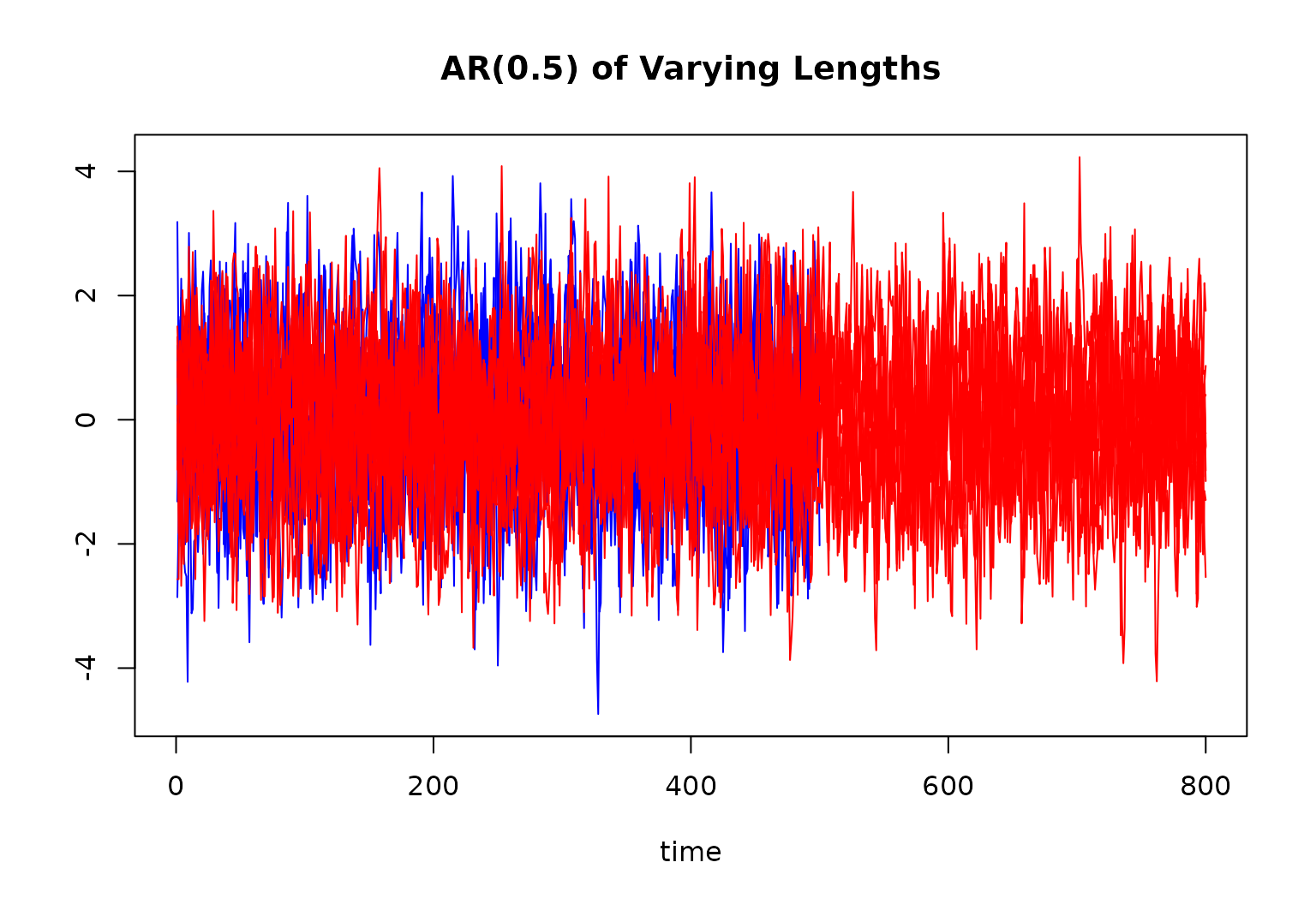
"ARp" input to gen_data()
This input calls the generate_AR() function.
R = 20
# Time series of different lengths
n = c(rep(500, R/2), rep(800, R/2))
burn = 50

## `ARp` method:
tmp = gen_data(
  gen_method = "ARp",
  phi = c(0.5),
  n = n,
  R = R,
  burn = burn
 )

# extract time series
ts = tmp$ts_list

# extract true_phi
tp = tmp$true_phi

# plot the time series
## Create an empty plot
 plot(
   x = c(),
   y = c(),
   xlim = c(0, 800),
   ylim = range(ts),
   ylab = "",
   xlab = "time",
   main = "AR(0.5) of Varying Lengths"
 )
 for (r in 1:10) {
   lines(ts[[r]][, 1], col = "blue")
 }
 for (r in 11:R) {
   lines(ts[[r]][, 1], col = "red")
 }
True Spectral Density for ARp
full_spec <- matrix(data = NA, nrow = 1000, ncol = R)
omega <- seq(0, pi, length.out = 1000)
phi <- tp
for(r in 1:R){
  full_spec[,r] = arma_spec_vectorized(omega = omega, phi = phi)
}

matplot(x = omega,
        y = full_spec,
        type = "l",
        ylab = bquote(g(omega)),
        xlab = bquote(omega),
        lwd = 2)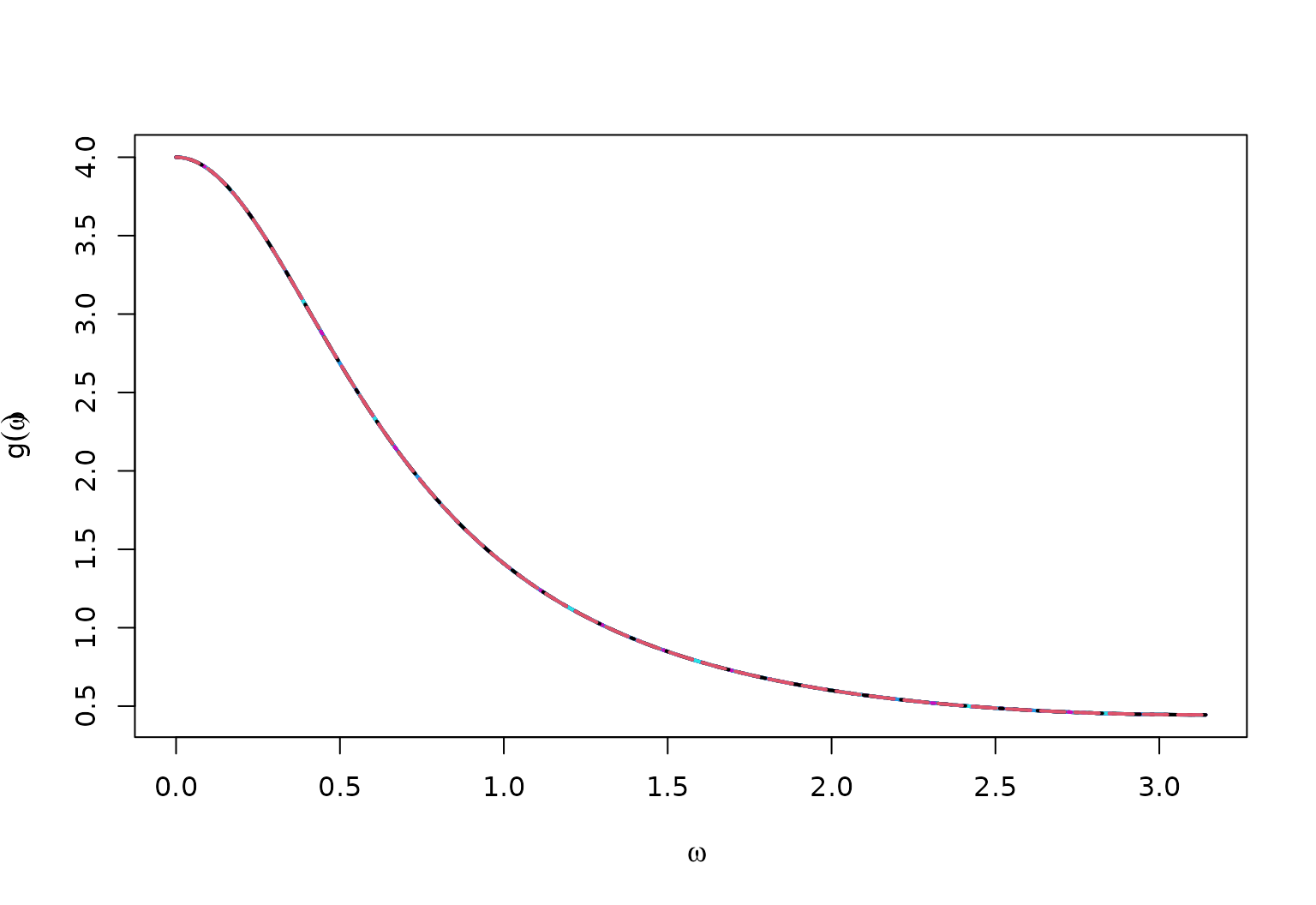
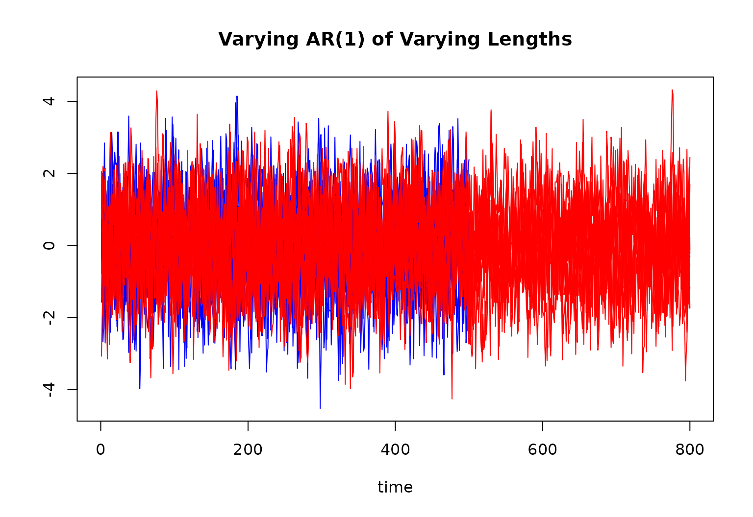
"AR1vary" input to gen_data()
This input calls the generate_AR1vary() function.
R = 20
# Time series of different lengths
n = c(rep(500, R/2), rep(800, R/2))
burn = 50

## `AR1vary` method:
 tmp <- gen_data(
   gen_method = "AR1vary",
   n = n,
   R = R,
   min = 0.45,
   max = 0.6,
   burn = burn
 )

# extract time series
ts = tmp$ts_list

# extract true_phi
tp = tmp$true_phi

# plot the time series
## Create an empty plot
 plot(
   x = c(),
   y = c(),
   xlim = c(0, 800),
   ylim = range(ts),
   ylab = "",
   xlab = "time",
   main = "Varying AR(1) of Varying Lengths"
 )
 for (r in 1:10) {
   lines(ts[[r]][, 1], col = "blue")
 }
 for (r in 11:R) {
   lines(ts[[r]][, 1], col = "red")
 }
True Spectral Density for AR1vary
full_spec <- matrix(data = NA, nrow = 1000, ncol = R)
omega <- seq(0, pi, length.out = 1000)
phi <- tp
for(r in 1:R){
  full_spec[,r] = arma_spec_vectorized(omega = omega, phi = phi[r])
}

matplot(x = omega,
        y = log(full_spec),
        type = "l",
        ylab = bquote("log("*g(omega)*")"),
        xlab = bquote(omega),
        lwd = 2)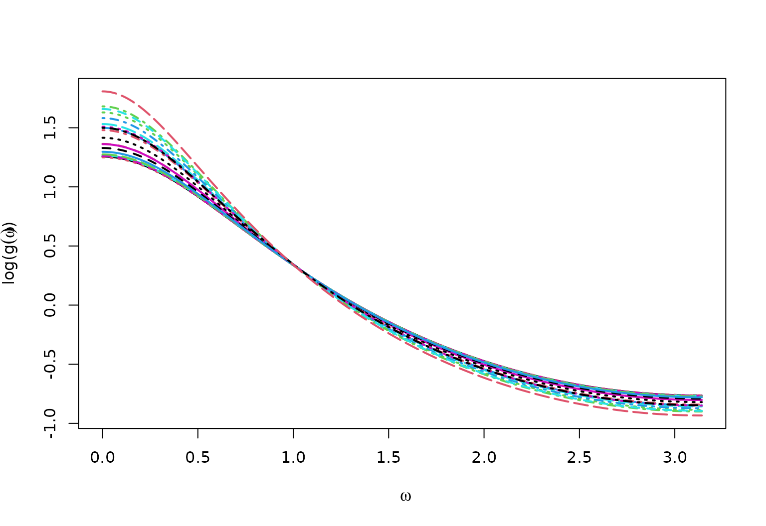
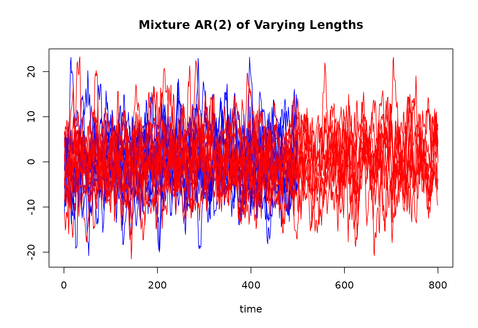
"AR2mix" input to gen_data()
This input calls the generate_AR2_mixture()
function.
## `AR2mix` method:
 R <- 20
# Time series of different lengths
n = c(rep(500, R/2), rep(800, R/2))

 peaks1 <- runif(R, min = 0.2, max = 0.23)
 bandwidths1 <- runif(R, min = .1, max = .2)
 peaks2 <- runif(R,
                 min = (pi * (2 / 5)) - 0.1,
                 max = (pi * (2 / 5)) + 0.1)
 bandwidths2 <- rep(0.15, R)
 peaks <- rbind(peaks1, peaks2)
 bandwidths <- rbind(bandwidths1, bandwidths2)

 tmp <- gen_data(
   gen_method = "AR2mix",
   peaks = peaks,
   bandwidths = bandwidths,
   n = n
 )

# extract time series
ts = tmp$ts_list

# extract out the phi1
phi1_true = tmp$phi1_true
# extract out the phi2
phi2_true = tmp$phi2_true

# plot the time series
## Create an empty plot
 plot(
   x = c(),
   y = c(),
   xlim = c(0, 800),
   ylim = range(ts),
   ylab = "",
   xlab = "time",
   main = "Mixture AR(2) of Varying Lengths"
 )
 for (r in 1:10) {
   lines(ts[[r]][, 1], col = "blue")
 }
 for (r in 11:R) {
   lines(ts[[r]][, 1], col = "red")
 }
True log Spectral Density for AR2mix
full_spec <- matrix(data = NA, nrow = 1000, ncol = R)
omega <- seq(0, pi, length.out = 1000)

# Calculate the SDF for generated data:
for(r in 1:R){
  g = rep(0, length(omega))
  for(p in 1:nrow(phi1_true)){
    g = g + arma_spec_vectorized(omega, phi = c(phi1_true[p,r], phi2_true[p,r]))
  }
  full_spec[,r] = g
}

matplot(x = omega,
        y = log(full_spec),
        type = "l",
        ylab = bquote("log("*g(omega)*")"),
        xlab = bquote(omega),
        lwd = 2)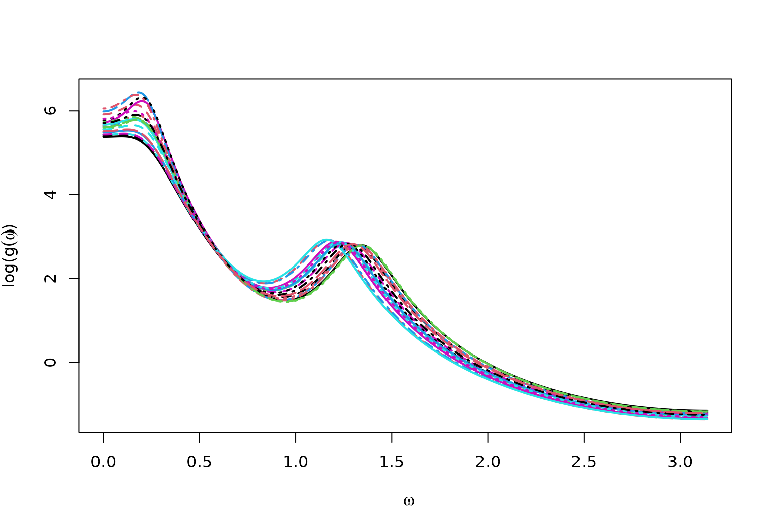
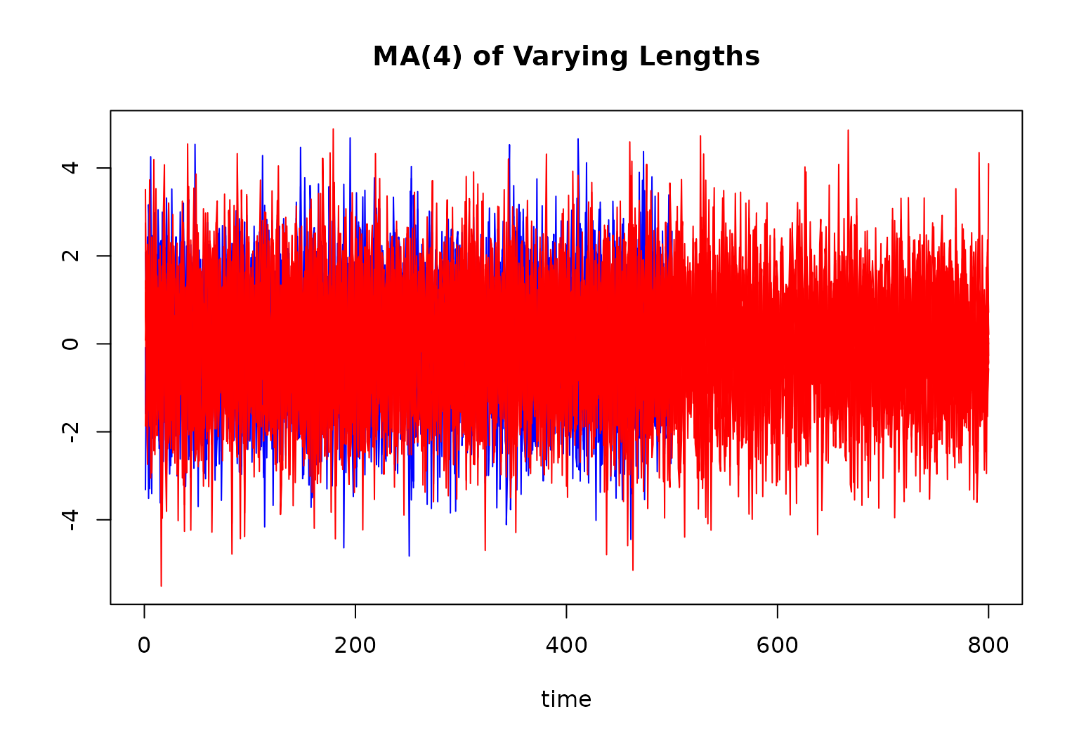
"MA4" input to gen_data()
This input calls the generate_MA4() function.
R = 20
# Time series of different lengths
n = c(rep(500, R/2), rep(800, R/2))
burn = 50

## `MA4` method:
 tmp <- gen_data(
   gen_method = "MA4",
   n = n,
   R = R,
   burn = burn
 )

# extract time series
ts = tmp$ts_list

# extract true_phi
tp = tmp$true_theta

# plot the time series
## Create an empty plot
 plot(
   x = c(),
   y = c(),
   xlim = c(0, 800),
   ylim = range(ts),
   ylab = "",
   xlab = "time",
   main = "MA(4) of Varying Lengths"
 )
 for (r in 1:10) {
   lines(ts[[r]][, 1], col = "blue")
 }
 for (r in 11:R) {
   lines(ts[[r]][, 1], col = "red")
 }
True Spectral Density for MA4
full_spec <- matrix(data = NA, nrow = 1000, ncol = R)
omega <- seq(0, pi, length.out = 1000)
theta <- tp
for(r in 1:R){
  full_spec[,r] = arma_spec_vectorized(omega = omega, theta = theta[,r])
}

matplot(x = omega,
        y = log(full_spec),
        type = "l",
        ylab = bquote("log("*g(omega)*")"),
        xlab = bquote(omega),
        lwd = 2)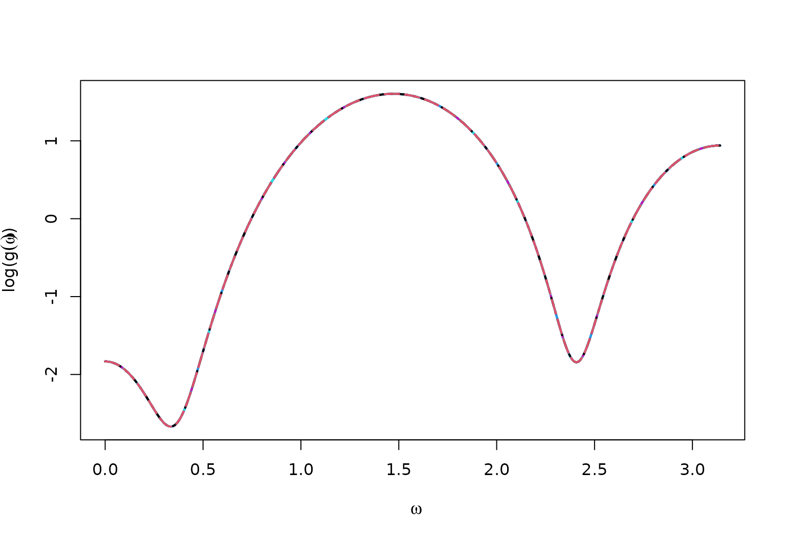
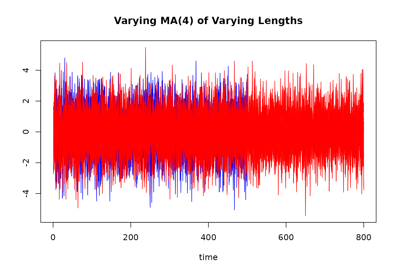
"MA4vary" input to gen_data()
This input calls the generate_MA4vary() function.
R = 20
# Time series of different lengths
n = c(rep(500, R/2), rep(800, R/2))
burn = 50

## `MA4vary` method:
 alpha <- 0.05
 tmp <- gen_data(
   gen_method = "MA4vary",
   n = n,
   R = R,
   burn = burn,
   alpha = alpha
 )

# extract time series
ts = tmp$ts_list

# extract true_phi
tp = tmp$true_theta

# plot the time series
## Create an empty plot
 plot(
   x = c(),
   y = c(),
   xlim = c(0, 800),
   ylim = range(ts),
   ylab = "",
   xlab = "time",
   main = "Varying MA(4) of Varying Lengths"
 )
 for (r in 1:10) {
   lines(ts[[r]][, 1], col = "blue")
 }
 for (r in 11:R) {
   lines(ts[[r]][, 1], col = "red")
 }
True Spectral Density for MA4vary
full_spec <- matrix(data = NA, nrow = 1000, ncol = R)
omega <- seq(0, pi, length.out = 1000)
theta <- tp
for(r in 1:R){
  full_spec[,r] = arma_spec_vectorized(omega = omega, theta = theta[,r])
}

matplot(x = omega,
        y = log(full_spec),
        type = "l",
        ylab = bquote("log("*g(omega)*")"),
        xlab = bquote(omega),
        lwd = 2)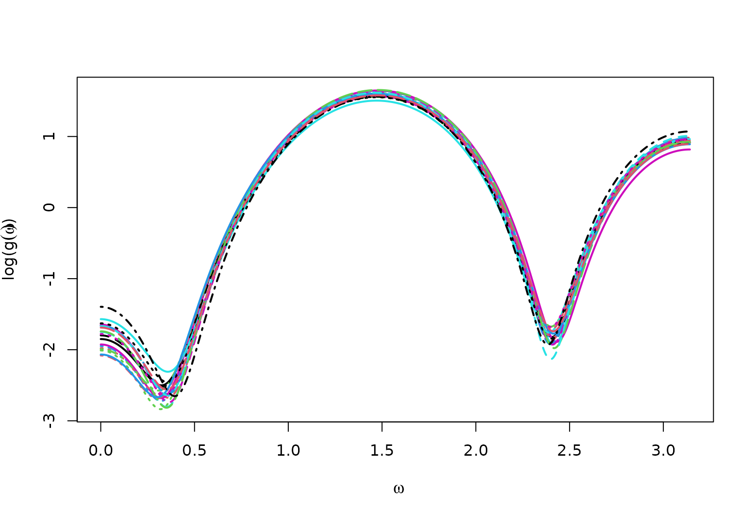
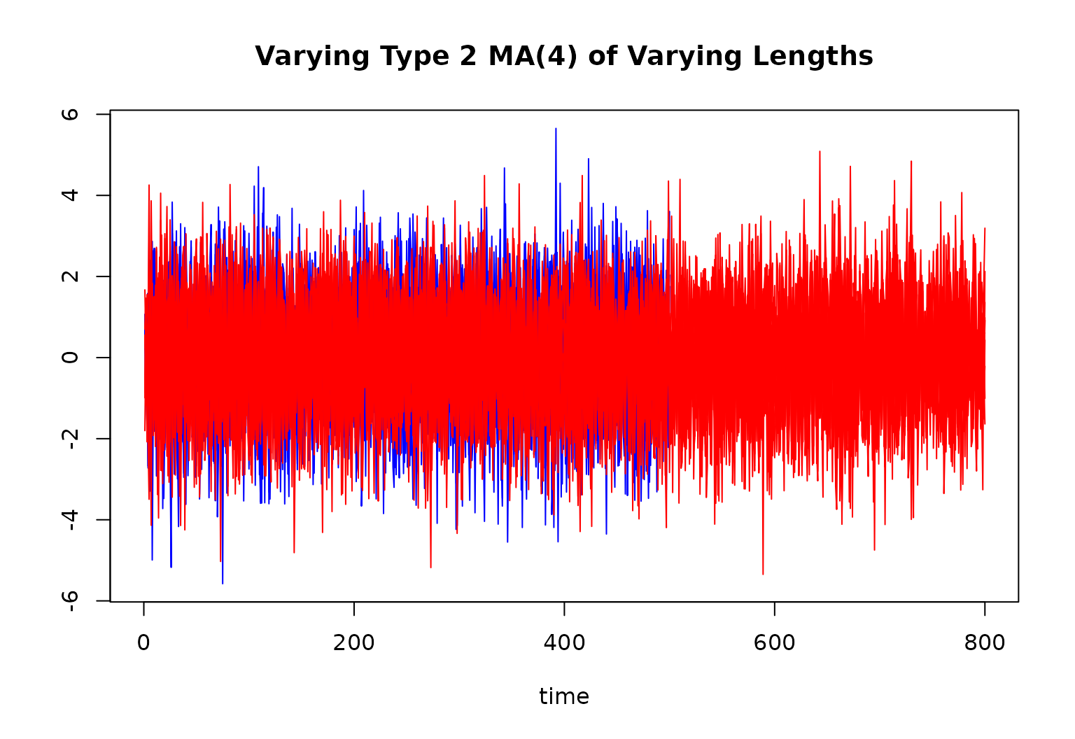
"MA4varyType2" input to gen_data()
This input calls the generate_MA4varyType2()
function.
R = 20
# Time series of different lengths
n = c(rep(500, R/2), rep(800, R/2))
burn = 50

## `MA4vary` method:
 alpha <- 0.5
 tmp <- gen_data(
   gen_method = "MA4varyType2",
   n = n,
   R = R,
   burn = burn,
   alpha = alpha
 )

# extract time series
ts = tmp$ts_list

# extract true_phi
tp = tmp$true_theta

# plot the time series
## Create an empty plot
 plot(
   x = c(),
   y = c(),
   xlim = c(0, 800),
   ylim = range(ts),
   ylab = "",
   xlab = "time",
   main = "Varying Type 2 MA(4) of Varying Lengths"
 )
 for (r in 1:10) {
   lines(ts[[r]][, 1], col = "blue")
 }
 for (r in 11:R) {
   lines(ts[[r]][, 1], col = "red")
 }
True Spectral Density for MA4varyType2
full_spec <- matrix(data = NA, nrow = 1000, ncol = R)
omega <- seq(0, pi, length.out = 1000)
theta <- tp
for(r in 1:R){
  full_spec[,r] = arma_spec_vectorized(omega = omega, theta = theta[,r])
}

matplot(x = omega,
        y = log(full_spec),
        type = "l",
        ylab = bquote("log("*g(omega)*")"),
        xlab = bquote(omega),
        lwd = 2)