generate R-many conditionally independent varying MA(4) time series

generate_MA4_vary() generates R-many time series where the MA(4) that is used as the base coefficients for the variation is (-.3,-.6,-.3,.6). This is based on the MA(4) used in Granados-Garcia et al. (2022) .

Usage

generate_MA4_vary(n, R = 1, burn = 50, alpha = 0.05)

Arguments

n: A numeric vector that determines the length of the time series generated. Must contain R-many entries. Time series may be of different lengths.
R: An optional scalar indicating the number of conditionally independent time series to be generated. (default is 1).
burn: A scalar indicating the amount of burn-in to be used with stats::arima.sim(). (default is 50).
alpha: A scalar specifying the variation wanted from the base coefficients. (default is 0.05).

Value

The function returns a list containing:

`ts_list`	returns an `R`-long list each containing an `(n[r]` \(\times\) `1)` matrix of the generated time series.
`true_theta`	returns a `(4` \(\times\) `R)` matrix of true generated MA(4) coefficients.
`alpha`	returns the user-provided variation scalar.
`mu_r_gen`	returns the `(4` \(\times\) `R)` matrix of the generated standard normal values used to help calculate the new MA(4) coefficients.

Details

The variation around the base theta coefficients is generated in the function by:

Sample 4 values from a \(N(0,1)\) to use as a "mean".
Calculate: basetheta + alpha * mu_r * abs(basetheta) where basetheta is the original coefficients; mu_r is the 4 sampled values from the \(N(0,1)\); and alpha is the user-specified scalar that controls the variation around the base coefficients.
Generate: A new time-series using the new theta value from step 2.
Repeat steps 1-3 R-many times.

Examples

R <- 20
## For time series of different lengths:
n <- c(rep(500, R/2), rep(800, R/2))
burn <- 50
alpha <- 0.05
ts <- generate_MA4_vary(n = n, R = R, burn = burn, alpha = alpha)$ts_list

## The function returns an R-long list object each with a (n[r] x 1) matrix object,
## a (4 x 20) matrix of true MA(4) coefficients,
## a scalar returning the alpha provided,
## and a (4 x 20) matrix of the standard normal values generated for each R.

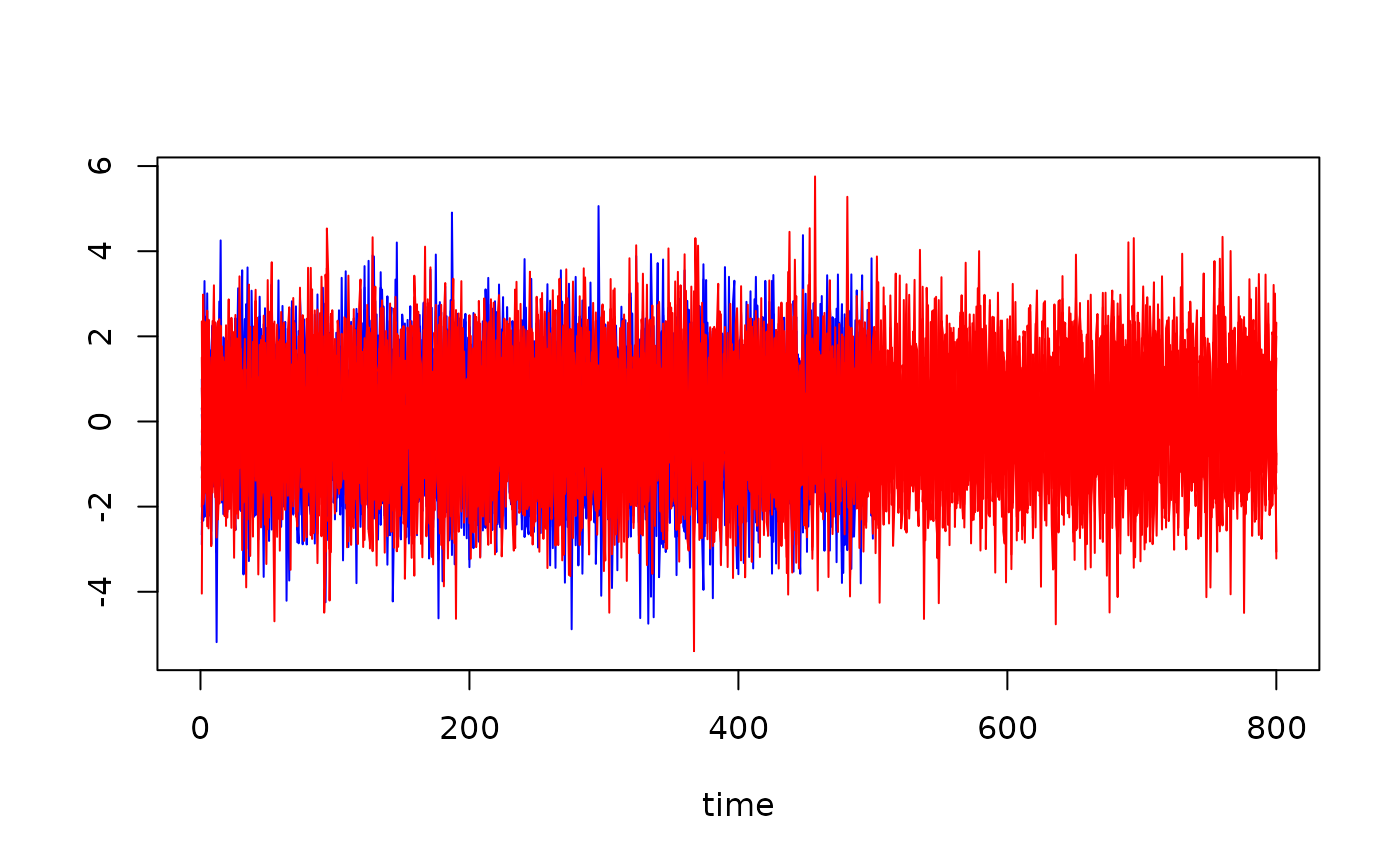
## Plot
## Create an empty plot
plot(
  x = c(),
  y = c(),
  xlim = c(0, 800),
  ylim = range(ts),
  ylab = "",
  xlab = "time"
)
for (r in 1:10) {
  lines(ts[[r]][, 1], col = "blue")
}
for (r in 11:R) {
  lines(ts[[r]][, 1], col = "red")
}